In this post, we’re going to finish the work started in the previous one and eventually classify the quantized version of Wrist-worn Accelerometer Dataset. There are many ways to classify the datasets with numerical features, but the Decision Tree algorithm is one of the most intuitively understandable and simple approaches in terms of its underlying implementation. We are going to build a Decision Tree classifier using Numpy library and generalize it to Random Forest — an ensemble of randomly generated trees that is less prone to the data noise.

TL;DR: As always, here is a link to the repository with solutions implementing Decision Tree and Random Forest classifiers, as well as their training using the accelerometer dataset.

Decision Trees

A decision tree is a classifier expressed as a recursive partition of the analyzed dataset. Mathematically, it represents a function that takes as input a vector of attribute values and returns a “decision” — a single output value. The tree reaches its decision by performing a sequence of tests on a given observation attributes. Each internal node in the tree corresponds to a test of the value of one of the observation’s attributes $A_i$, and the branches from the node are labeled with the possible values of the attribute $A_i = v_{ik}$. Every leaf node in the tree specifies a value to be returned by the function.

However, in the post we’re describing a bit simplified version of this general conception. Figure 1 shows a graphical representation of a decision tree classifier we’re going to implement. This specific tree was trained on Wine Dataset. The dataset is exceptionally tiny and contains only 178 instances, each belongs to one of the 3 classes. These properties make it an ideal candidate for a smoke or sanity test when developing the machine learning code. Even the simplest classifier should show an excellent performance on it, and the training process is very very fast. In our case, each node has the two branches only and makes its decision comparing attribute like Magnesium with a threshold value. Therefore, even for the continuous attributes, each node performs a binary classification task.

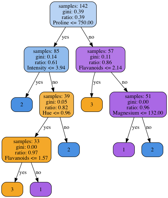Fig 1. An example of decision tree trained on Wine Dataset

The figure gives a clue why the considered method of classification contains the word “tree” in its name. The decision process constitutes the following branches of the directed acyclic graph depending on the values of a classified observation’s attributes.

Note: The pseudo-code that goes below is nor a standard definition of Decision Tree algorithm, neither a novel implementation. It is intended to provide a concise and intuitively clear explanation of the generic idea which I would like to have when started working on my implementation. Here is a link to the one of the original papers on decision trees.

Now when we’ve seen a visual representation of a trained classifier, the question is how can we formally represent the training process? As it was already mentioned, we’re discussing one of the purest versions of the Decision Tree algorithm implementation, as the pseudo-code shows.

def decision_tree(D: Dataset, depth: int) -> Node:
    if depth >= THRESHOLD:
        return majority_class(D)

    if empty(D):
        return None

    best_split = None
    for feature in features(D):
        for value in unique(feature):
            split = select_samples_less_or_equal(value, dataset=D)
            quality = compute_quality(split, D, classes(D))
            if better(quality, best_split):
                best_split = quality
     
    D_left, D_right = split(D, bestSplit)
    left_child = decision_tree(D_left, depth + 1)
    right_child = decision_tree(D_right, depth + 1)
    node = create_node(left_child, right_child)
    return node            

We’re building a decision tree by recursively splitting the dataset into two subsets based on the values of its attributes. One of the crucial algorithm points is the call of the compute_quality() function that estimates how “good” (in terms of the classification accuracy) the partition is. Note that we also limiting the depth of a tree. Otherwise, we could get a very deep tree with just a few observations per node. Therefore, as soon as we’re reaching the maximal depth we are returning the most frequent class of the subset.

There are several possible quality metrics. One of this metrics is called Gini impurity score and is defined with the formula:

$$ Gini(D, C) = N \times \left[ 1 - \sum_{c_j \in C}\left(\frac{1}{N}\sum_{y_i \in D}{I(y_i = c_j)}\right)^2 \right] $$

where $N$ is the total number of the samples in the dataset $D$, and $I$ denotes an indicator variable which is equal to 1 when the $j$th instance’s class is equal to $c_j$, and is equal to 0 — otherwise.

As it follows from the definition, the Gini score shows how impure the split is. The higher the score, the worse a specific split, the more various classes are represented in the child nodes after a split. Therefore, this metric is an opposite of the quality, and our goal is to achieve the lowest possible Gini score when splitting a parent node.

In the next section, we’re going to build a simple decision tree implementation that works with continuous attributes.

Decision Tree Implementation with Numpy

The snippet below shows a simple implementation of the Decision Tree learning algorithm. There are a few other improvements shown in the Python script that are not present in the pseudo-code discussed below.

The code is mostly self-explanatory, but there is a couple of tips. First of all, reaching the maximally allowed depth is not the only considered “shortcut” condition. Lines 87-90 are also checking if all observations belong to a single class and if the node contains too few observations to be split again. Second, the implementation doesn’t split the original 2D array into smaller arrays but operates with indexes instead to be more memory efficient. Finally, the tree learning function provides an opportunity to use only a subset of features to build the tree. Why do we need such functionality? Isn’t it better to always use all available attributes of the data? The reason is described in the next section.

Ensemble Methods and Random Forests

Ok, now we have an implemented classifier and can use it to classify various datasets. However, what’s going on if we try to train a tree on various subsets of the original dataset? The Figure 2 shows the decision trees trained on three distinct random splits of the dataset.

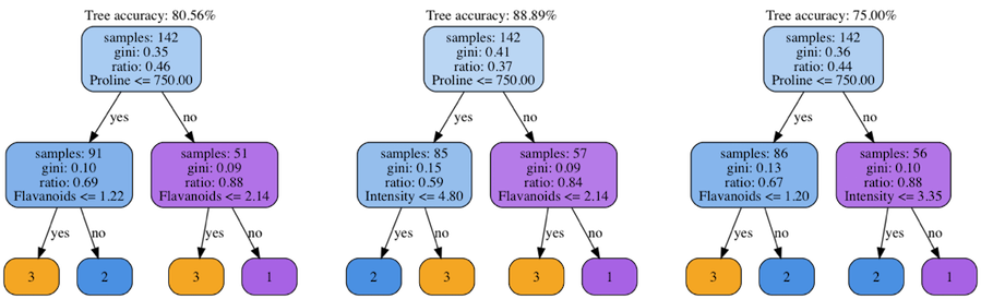Fig 2. Group of decision trees trained using different dataset splits

Despite that the root nodes are almost equal, the trees are a bit different in their leaves and the inner nodes. It means that you’re going to get different classification results with every new random generator seed. Moreover, the classifier’s accuracy significantly changes from one tree to another. The reason directly follows from the tree’s construction process. When taking various subsets of the original dataset, we’re effectively changing the list of considered feature values when building the nodes. Therefore, with every start we have a bit different Gini score and different best splits.

How can we alleviate this issue? One of the possible solutions is to build several trees and average their predictions. The theoretical foundation of this result comes from the theorem about weak learners. Briefly speaking, the idea is that if one has a classifier that performs a bit better then a random one (like better than a fair coin in case of binary classification data), then having a sufficient number of such weak classifiers would be able to predict the classes with almost perfect accuracy. Strictly speaking, to apply the theorem the dataset samples should meet a requirement of being independent and identically distributed random variables, and the distribution where samples come from shouldn’t change much. Nevertheless, this approach works reasonably well on practice if each classifier’s training process is a bit different from the another one.

So now it is time to answer the question we’ve stated in the previous section: Why to build a tree using only a subset of features? To make trees as different from each other as possible. In this case, every tree makes different kinds of mistakes, and when averaged they could give us better accuracy than one by one.

The idea of the joining a group of weak learners into a single strong one could be applied not only to the Decision Tree but to any kind of “weak” classifier. In the cases when this approach is applied to a group of trees, the strong learner is called Random Forest.

The snippet below shows a simple wrapper build on top of our decision tree implementation which creates a bunch of decision trees and provides a few convenience methods for making the predictions.

Lines 28-36 create an array of decision trees. Every tree is trained on a bootstrapped sample of the original dataset. Lines 46-66 define the method called predict_proba() returning a matrix with classes occurrence frequencies based on the trees predictions. Other methods and utilities serve for convenience purposes. The standalone implementation of the classifier and the helping utilities can be found here.

Now we’re ready to join everything described in this post together and apply our DIY classifiers to the Wrist-worn Accelerometer Dataset.

Accelerometer Dataset Classification

As we know from the previous post, the accelerometer dataset is not prepared to be directly fed into a classical supervised learning algorithm that expects an array with samples $X$ and an array with targets $y$. Therefore, the first step is to apply the dataset quantization algorithm. Then, we need to convert targets from strings into numerical values. Next, we split the quantized dataset into the training and validation subsets. Finally, we’re training an instance of a Random Forest classifier on the training subset and checking its performance on the validation subset.

The snippet below shows all these steps. An interested reader could also check this Jupyter notebook that contains the same steps, and can be used as a playground to investigate separate steps of our pipeline.

A question that one would ask when using an ensemble classifier is how many weak learners do we need to use to achieve the best possible performance? One way to know it is to add classifiers one after another to the ensemble and check the ensemble’s performance. Figure 3 shows a plot showing the dependency between a logarithm of the number of trees $N$ in the ensemble and the validation accuracy measured in percents. The $N$ value is varied from $1$ to $1000$. Each orange dot reflects an accuracy for a specific $N$ value, and the blue curve is a polynomial approximation of these discrete measurements.

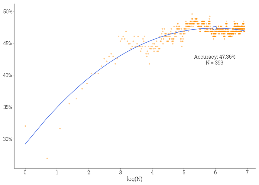Fig 3. Relationship between ensemble accuracy and its size

We’re getting approximately 47% of accuracy on the validation subset with 14 classes, and we can claim that our classifier successfully grasps the relationships between samples and targets, performing much better than a random guess.

As the curve shows, we’re getting a significant accuracy increase when going from a single tree to several dozens of trees. However, the ensemble accuracy has the boundary. The accuracy slowly stops increasing when the number of trees reaches several hundred. To get better results, we could try to randomize the training process even more, add more features, or gather extra data.

Conclusion

Decision trees and their ensembles are intuitively clear but powerful machine learning techniques. There are many improvements to the original algorithm and a bunch of great libraries that allow training trees ensembles in parallel fashion and getting higher accuracy, like, an excellent library called XGBoost. Nevertheless, even a naïve implementation shows decent results and proofs that it is not too challenging to implement a machine learning classifier from scratch.